import numpy as np
import scipy as sp  # Subpackages still need to be imported individually
import matplotlib.pyplot as plt
from matplotlib import cm
import tables
import h5py
# For website
%matplotlib inline
Python: the language for effective scientific computing
Ross Barnowski rossbar@berkeley.edu | @rossbar on GitHub
DOE Python Exchange | 12/01/2021
A bit about me…
I began my research career in the national lab system:
Summer 2008: SULI internship at Argonne National Laboratory
Summer 2009: Summer internship with the Nuclear Data Group at LLNL
First exposure to Python
2010-2019: Grad school -> post-doc -> research scientist & lecturer
UC Berkeley nuclear engineering department & the Applied Nuclear Physics group at LBNL
I’m a nuclear engineer by training, specializing in radiation instrumentation; particularly gamma-ray spectroscopy and imaging.
Open-source software, specifically scientific Python, was the key component in my research projects.
Real-time 3D gamma-ray mapping
Scene data fusion (SDF): computer vision + gamma-ray imaging
Applications in e.g. nuclear contamination remediation
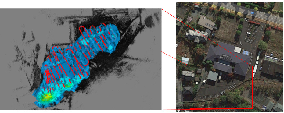
Right: Aerial view of measurement area. Left: 3D gamma-ray image reconstruction — Red line = path of imager through the scene, B/W dots = 3D point cloud model of the scene, Heatmap = image reconstruction; color scale corresponds to relative reconstructed intensity.
Volumetric gamma-ray imaging
Imaging modalities for e.g. nuclear safeguards or small-animal imaging

Demonstration of Compton imaging for applications in small animal molecular imaging. Left: A Cs-137 calibration source in the shape of a thin rod mounted on a rotating stage. Right: Three projections of reconstructed image from a tomographic measurement.
My background
Systems integration
Interfacing with hardware, data acquisition systems
Synchronizing & fusing data from disparate sources
Real-time acquisition and analysis
Distributed computing: performance, load-balancing
Workstation-scale computing
Mobile (hand-held or cart-based) measurement systems
Datasets usually O(GB) - not big data
On to the question: Why Python?
General-purpose language: can address a wide range of problems & computational tasks
Optimizes developer time
Effective language for the communication of scientific ideas
Community-based development model!
General purpose programming language
[This is] a distinguishing feature of Python for science and one of the reasons why it has been so successful in the realm of data science: instead of adding general features to a language designed for numerical and scientific computing, here scientific features are added to a general-purpose language. This broadens the scope of problems that can be addressed easily, expands the sources of data that are readily accessible and increases the size of the community that develops code for the platform.
Scipy 1.0: fundamental algorithms for scientific computing in Python
* Emphasis mine
See also: Jim Hugunin’s position paper laying out the motivation
and design principles for Numeric (ancestor of NumPy) in 1995(!)
Integrating with other languages
Performance - e.g. writing performance-critical chunks in low-level languages
Extending - adding custom algorithms or data structures (e.g.
ndarray)
Wrapping - providing convenient, high-level interfaces to existing low-level code
Common in e.g.
scipy(BLAS, Eigen, etc.)Legacy code and software from vendors, e.g. commercial hardware
A fundamental feature of Python, and many additional tools to fit various use-cases:
Cython, Pythran, numba, PyBind11, …
#include <Python.h>
#include "numpy/arrayobject.h" // provides the numpy C API

...  // Defining all the wrapper functions

static PyMethodDef SISMethods[] = {
    {"connectToDAQ", (PyCFunction)wrap_connectToDAQ, METH_VARARGS, "Connect to SIS3150"},
    {"configuration", (PyCFunction)wrap_configuration, METH_VARARGS, "Configure SIS3302"},
    {"startacquisition", (PyCFunction)wrap_startacquisition, METH_VARARGS, "Start SIS3302"},
    {"stopacquisition", (PyCFunction)wrap_stopacquisition, METH_VARARGS, "Stop SIS3302"},
    {"acquiredata", (PyCFunction)wrap_acquiredata, METH_VARARGS, "Acquire data from SIS3302"},
    {"acquireDataWithRaw", (PyCFunction)wrap_acquireDataWithRaw, METH_VARARGS, "Acquire edata and rdata from SIS3302"},
    {NULL,NULL}
};

PyMODINIT_FUNC initsis(void) { // must be init<modulename> (init_cext => _cext)
    (void) Py_InitModule("sis", SISMethods);
    import_array(); // load numpy (effectively "import numpy") for use in this module
};
Original wrapping work by Cameron Bates (@crbates), now at LANL, whom I credit with convincing me of the value of the Python C/API!
import time
from SIS import sis

class SISDAQThread:
    def __init__(self, config_file):
        self.hardware_started = False
        self.paused = True  # state controlled via GUI button press
        # Initialize hardware communication
        sis.connectToDAQ()
        sis.configuration(config_file)

    def run(self):
        if not self.hardware_started and not self.paused:
            self.start_hardware()

        if self.hardware_started and not self.paused:
            timestamps, energies, channel_nos, trigger_values = sis.acquiredata()

        # Validation + send to other processes for analysis

    def start_hardware(self):
        sis.startacquisition()
        self.start_time = time.time()
        self.hardware_started = True
Incorporate into scripts, local GUIs, Web-UI
Instantly gained platform-independence
Optimize Developer time
Syntactically, Python code looks like executable pseudo code. Program development using Python is 5-10 times faster than using C/C++… Often, [a prototype program] is sufficiently functional and performs well enough to be delivered as the final product, saving considerable development time.
Not to mention the time it takes to become proficient in the language!
Powerful operations via simple, expressive syntax
Incremental approach to data analysis
Identify and address bottlenecks sequentially
Simple path(s) for scaling up to larger problems
Example: Digital signal processing for gamma-ray spectroscopy
with tables.open_file("_data/digitized_preamp_signals.h5") as hf:
    signal = hf.root.signals[0, ...]

fig, ax = plt.subplots()
ax.plot(signal)
ax.set_title("Digitzed raw signal from a radiation spectrometer")
ax.set_ylabel("Amplitude (ADC units [arbitrary])")
ax.set_xlabel("Sample # $10 \frac{ns}{sample}$");
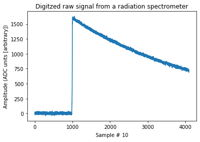
Signal amplitude reflects total deposited energy
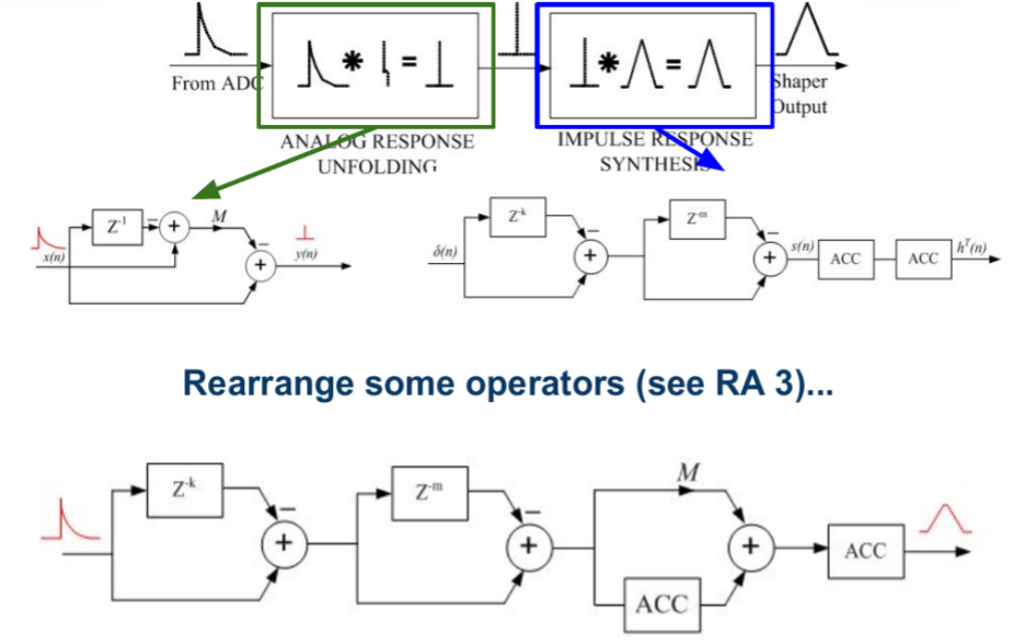
Algorithm described in Digital synthesis of pulse shapes in real time for high resolution radiation spectroscopy by Valentin Jordanov (pdf link)
Simple operations: multiplication, addition, accumulation, delays (Z-n)
Select values for the parameters:
k = 450  # "Peaking time", in sample units (i.e. 4.5 microseconds)
m = 60  # "Gap time", in sample units (i.e. 600 nanoseconds)
M = 3600  # Estimate of exponential decay constant in sample units
Implement signal delay with slicing:
s = signal[:-(2*k+m)]
sk = signal[k:-(m+k)]
skm = signal[k+m:-k]
s2km = signal[2*k+m:]
Apply shaper:
S1 = ((s - sk) + (s2km - skm)).astype(np.int64)
S2 = M * S1 + np.cumsum(S1)
shaped = np.cumsum(S2)
A little cleanup:
# Pad result for time-alignment with input signal
shaped = np.hstack((np.zeros(2*k+m), shaped))

# Gain compensation
shaped /= M*k
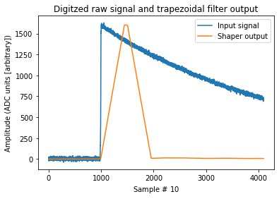
How’d we do?
fig, ax = plt.subplots()
ax.plot(signal, label="Input signal")
ax.plot(shaped, label="Shaper output")
ax.set_title("Digitzed raw signal and trapezoidal filter output")
ax.set_ylabel("Amplitude (ADC units [arbitrary])")
ax.set_xlabel("Sample # $10 \frac{ns}{sample}$")
ax.legend();
Scaling up
Scaling the analysis up to multiple signals is straightforward thanks to broadcasting:
def trapezoidal_shaper(signals, k, m, M):
    signals = np.atleast_2d(signals)  # Each row represents a single measurement
    # Apply delays to all signals
    s = signals[..., :-(2*k+m)]
    sk = signals[..., k:-(m+k)]
    skm = signals[..., k+m:-k]
    s2km = signals[..., 2*k+m:]
    # Apply shaper operations along appropriate axis
    S1 = ((s - sk) + (s2km - skm)).astype(np.int64)
    S2 = M * S1 + np.cumsum(S1, axis=1)
    shaped = np.cumsum(S2, axis=1)
    # Time-alignment and gain correction
    shaped = np.hstack((np.zeros((signals.shape[0], 2*k+m)), shaped))
    shaped /= M * k
    return shaped
# Load
with tables.open_file("_data/digitized_preamp_signals.h5", "r") as hf:
    print(f"Total number of signals in file: {hf.root.signals.shape[0]}")
    signals = hf.root.signals.read()

# Analyze
shaped = trapezoidal_shaper(signals, k, m, M)
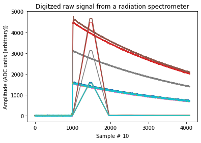
Total number of signals in file: 1104
# Visualize
fig, ax = plt.subplots()
ax.plot(signals[:10].T)
ax.plot(shaped[:10].T)
ax.set_title("Digitzed raw signal from a radiation spectrometer")
ax.set_ylabel("Amplitude (ADC units [arbitrary])")
ax.set_xlabel("Sample # $10 \frac{ns}{sample}$");
Takeaways
Implementation of analysis is very near the original algorithm
Incremental approach: explore/test with subset, easily scale up
A quick aside on interoperability
import dask.array as da

# Data still on disk
data = h5py.File("_data/digitized_preamp_signals.h5")["/signals"]

chunked_signals = da.from_array(data, chunks=(276, 4096))
chunked_signals
|
# Note: Calling a function full of *numpy* functions on a *dask array*
shaped = trapezoidal_shaper(chunked_signals, k, m, M)
shaped
|
Our analysis works on a new, non-numpy array object out-of-the-box! No changes/explicit conversions required!
This works because Dask implements protocols provided by NumPy for interoperability with array objects.
For more information, see e.g. NEP 18, which describes the __array_function__ protocol.
An effective language for communicating STEM concepts

An equation for list-mode maximum likelihood expectation maximization (MLEM)
Or, in NumPy:
def compute_em_iteration(λ, α, s):
    term_one = 1 / (α @ λ)
    term_two = α.T @ term_one
    return (λ / s) * term_two
and of course, it’s executable!
Example: Gamma-ray image reconstruction
Compton imaging is a specific modality of gamma-ray imaging
Based on the physics of gamma-ray scattering
Some fun quirks of this modality
Each photon interaction results in a cone in the imaging space
No lensing or collimation, inherently wide field-of-view
We’ll use a simulated dataset that contains 100 photon interactions from a gamma-ray source directly in front of a Compton camera
import scipy.sparse
fname = "_data/system_matrix_100cones_4piSpace_simulated_5degConeOpenAngle.h5"
img_shape = (181, 361)  # 4-pi imaging
with tables.open_file(fname, "r") as hf:
    system_matrix = sp.sparse.csr_matrix(hf.root.sysmat.read())
system_matrix
<100x65341 sparse matrix of type '<class 'numpy.float32'>'
	with 2378244 stored elements in Compressed Sparse Row format>
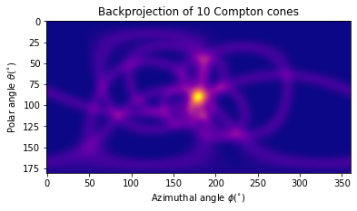
Let’s take a look at a few of the cones to get a sense for what the image looks like:
subset = np.ravel(system_matrix[:10].sum(axis=0))  # Sum of 10 backprojected cones

# Visualize
fig, ax = plt.subplots()
ax.imshow(subset.reshape(img_shape), cmap=cm.plasma)
ax.set_title("Backprojection of 10 Compton cones")
ax.set_xlabel("Azimuthal angle $\phi (^{\circ})$")
ax.set_ylabel("Polar angle $\\theta (^{\circ})$");
Now let’s try our ML-EM reconstruction technique:
# Use the backprojection to initialize the reconstruction
img = np.ravel(system_matrix.sum(axis=0))
initial_img = img.copy()  # Pre-reconstruction, for comparison
sensitivity = 1.0  # Ignore sensitivity for this simple example
n_iter = 10

for _ in range(n_iter):
    img = compute_em_iteration(img, system_matrix, sensitivity)
A quick qualitative comparison:
fig, ax = plt.subplots(1, 2, figsize=(16, 4))

for a, im, t in zip(ax, (initial_img, img), ("Backprojection", "Reconstruction")):
    a.imshow(im.reshape(img_shape), cmap=cm.plasma)
    a.set_title(t)
fig.tight_layout()

Takeaways
Scientific Python is excellent for communicating scientific ideas
Minimal language cruft
“Executable pseudo-code”
Reproducibility and extensibility
Readability is important!
Community
The secret-sauce of scientific Python
The user-contributor model
User input inherently a top priority
Strong connection between development and usage
Coherence
Projects built from or extend from same fundamental elements (e.g.
ndarray)Interoperablity!
Similar development practices amongst projects
Scientific Python Ecosystem
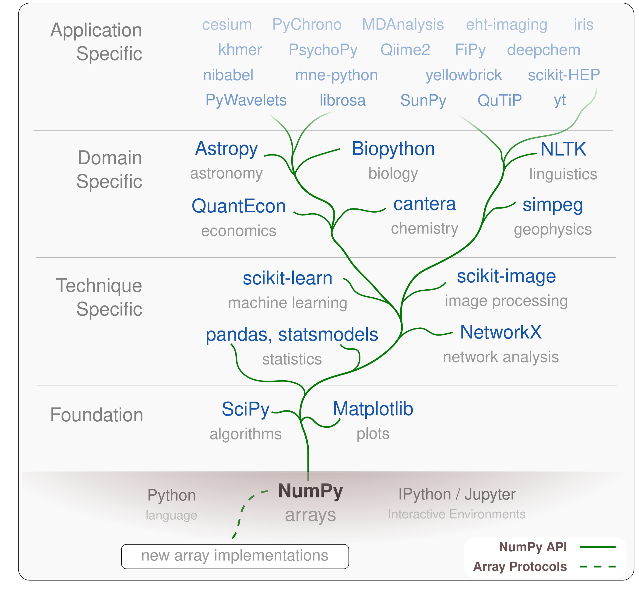
Projects built from or extend from same fundamental elements (e.g.
ndarray)Interoperablity!
Similar development practices
Sustainability?
A Healthy Ecosystem
An initiative to ensure the sustainable growth of the ecosystem moving forward:
https://scientific-python.org/
Discussion
Cross-project discussion forum: https://discuss.scientific-python.org/
Coordination
Mechanism for project coordination and loosely guiding ecosystem policy: Scientific Python Ecosystem Coordination documents (SPECs).
Growth
Getting the best tools into the hands of the most users!
The National Labs
The national labs have had a long history of developing and supporting open-source scientific Python
Numerical Python (aka
Numeric, predecessor to NumPy) - LLNL 90’s-00’sNetworkXgot it’s start at LANLMany, many others; including, but not limited to, Python (LFortran)
Another example: the SuperLU sparse matrix factorization package.
Developed and hosted by the national labs
Available in
scipy.sparse.linalg
Benefits users and the original researchers!
Removing barriers to contributing
Engaging with the wider scientific Python community: https://discuss.scientific-python.org/
Not everything belongs in scipy:
Lower the barrier for developing an ecosystem package
For new projects: development and community best-practices
Testing, documentation, releases, governance, etc.
Maintenance and sustainability
An idea (beta): https://rossbar.github.io/manual.scientific-python.org/